The full implementation is open-source:
The TL;DR
I built a system where a 3-DOF planar robot arm — a prismatic slider with two revolute joints — intercepts a ball thrown through 3D space, in real time. The robot only operates in a 2D plane, but the ball is a full 3D ballistic projectile. The trick: analytically compute when the ball will cross the robot's operational plane, lock that as a hard time horizon, and let a receding-horizon MPC figure out how to get the end-effector there.
The result: sub-centimetre interception accuracy at 20 Hz re-solve rates, with warm-started IPOPT converging in under 15 ms per cycle. The entire pipeline — trajectory estimation, MPC solve, motor command interpolation — runs inside a PyBullet physics loop at 240 Hz.
Why This Matters
Catching or intercepting fast-moving objects is one of those problems that sounds straightforward until you actually try it. The core tension: you need to plan a dynamically feasible trajectory for a multi-joint arm, but your planning horizon is dictated by the projectile — and that horizon is shrinking every millisecond.
Most prior work tackles this with high-DOF arms and full 3D workspaces. I wanted to explore a leaner setup: a planar PRR arm (Prismatic–Revolute–Revolute) that only moves in the XZ plane, intercepting a ball that travels through full 3D space. This constraint makes the problem harder in some ways (reduced workspace) and more tractable in others (the interception becomes a 2D terminal constraint).
The initial approach — treating interception time \(T^*\) as a free optimisation variable — worked for 2D in-plane throws. But the moment I introduced off-plane 3D trajectories, the solver started choking. That failure mode is what led to the key architectural insight of this project.
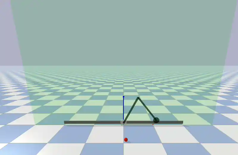
The Robot: A PRR Planar Arm on Rails
The manipulator is a 3-DOF planar arm defined in URDF and simulated in PyBullet:
| Joint | Type | Range | Role |
|---|---|---|---|
| Slider | Prismatic | \([-2, 2]\) m | Gross X-axis repositioning |
| Shoulder | Revolute | \([0.05, 2.0]\) rad | Arm elevation |
| Elbow | Revolute | \([-3.09, -0.05]\) rad | Reach fine-tuning |
Both links are 1.0 m, giving a max reach of 2.0 m from the shoulder. The slider extends the effective X workspace to roughly \([-4, 4]\) m. The entire URDF is spawned rotated \(\pi/2\) about the world X-axis so its native XY plane maps to the world XZ plane.
The forward kinematics are clean:
\[x_{ee} = q_0 + l_1 \cos(q_1) + l_2 \cos(q_1 + q_2)\]
\[z_{ee} = z_{base} + l_1 \sin(q_1) + l_2 \sin(q_1 + q_2)\]
where \(q_0\) is the slider position and \(z_{base} = 0.06\) m.
From Time-Optimal to Fixed-Time: Why \(T^*\) Broke Everything
My first MPC formulation treated the interception time \(T\) as a decision variable. The cost was:
\[J = 10T + 0.001 \| U \|^2\]
This worked well for in-plane throws (ball moving in XZ only). The solver would find the fastest feasible interception. But when I moved to 3D throws — ball originating at, say, \((4, 3, 1.5)\) with velocity \((-4, -3, 5)\) — things fell apart.
The failure mode: with \(T\) free, the solver had to simultaneously satisfy the terminal FK constraint and find a \(T\) where the ball actually intersects the arm's workspace. For off-plane balls, this coupling created over-constrained configurations. The ball's predicted position at time \(T\) is itself a function of \(T\) (ballistic trajectory), and the arm's reachable set at time \(T\) is also a function of \(T\) (through the dynamics). IPOPT would hit its iteration limit and return infeasible.
The fix was almost embarrassingly simple. The ball crosses the robot's XZ plane (\(Y = 0\)) at a deterministic time:
\[T_{cross} = \frac{-y_0}{v_y}\]
This is pure kinematics — no optimisation needed. Once I pulled \(T\) out of the decision variables and fixed the horizon to \(T_{cross}\), the problem became dramatically easier. The MPC now only asks: "Given exactly this much time, what's the minimum-effort trajectory to reach this point?"
The MPC Formulation
The solver is built once as a CasADi Opti problem and re-parameterised every cycle. Here's
the structure:
Decision variables:
- \(X \in \mathbb{R}^{6 \times (N+1)}\) — state trajectory \([q; \dot{q}]\)
- \(U \in \mathbb{R}^{3 \times N}\) — joint accelerations (controls)
Cost function:
\[J = \sum_{k=0}^{N-1} U_k^T W U_k + 10 \| \dot{q}_N \|^2\]
where \(W = \text{diag}(0.01, 1.0, 1.0)\). The asymmetric weighting is deliberate — the slider is cheap to accelerate (it's on rails), so the cost structure encourages the prismatic joint to absorb gross repositioning while the revolute joints handle fine alignment. The terminal velocity penalty ensures a smooth arrival.
Dynamics — Euler-discretised double integrator:
\[q_{k+1} = q_k + \dot{q}_k \cdot dt + \tfrac{1}{2} u_k \cdot dt^2\]
\[\dot{q}_{k+1} = \dot{q}_k + u_k \cdot dt\]
where \(dt = T_{remain} / N\) and \(N = 20\).
Terminal constraint — hard FK equality:
\[\text{FK}(q_N) = \begin{bmatrix} x_{ball} \\ z_{ball} \end{bmatrix}_{t = T_{cross}}\]
Box constraints at every node:
| Slider | Shoulder | Elbow | |
|---|---|---|---|
| Position | \([-2, 2]\) m | \([0.05, 2.0]\) rad | \([-3.09, -0.05]\) rad |
| Velocity | \(\pm 2.0\) m/s | \(\pm 5.0\) rad/s | \(\pm 5.0\) rad/s |
| Acceleration | \(\pm 4.0\) m/s² | \(\pm 10.0\) rad/s² | \(\pm 10.0\) rad/s² |
A note on the elbow bounds: the constraint \(q_2 \in [-3.09, -0.05]\) keeps the arm in elbow-up configuration and prevents full extension (\(q_2 \to 0\)), which would create a kinematic singularity where the Jacobian loses rank and the solver hits zero-gradient regions.
Trajectory Estimation and the Observation Window
Before the MPC fires, we need to know where the ball is going. I collect ~0.15 s of noisy ball observations (about 36 samples at 240 Hz) and fit three independent models via least-squares:
- X: linear — \(x(t) = x_0 + v_x t\)
- Y: linear — \(y(t) = y_0 + v_y t\)
- Z: quadratic — \(z(t) = z_0 + v_z t + \tfrac{1}{2} a t^2\)
The Z-axis gets a quadratic because gravity acts vertically. Gaussian noise (\(\sigma = 5\) mm) is injected into observations to stress-test robustness. Five samples is the hard minimum before the estimator returns anything.
From the fit, \(T_{cross}\) drops out immediately, and the ball's predicted \([x, z]\) at crossing gives us the terminal constraint target.
Receding Horizon: Closing the Loop
A single MPC solve at \(t = 0\) and open-loop execution is fragile. Estimation errors compound, the ball doesn't follow the model perfectly (PyBullet has its own integrator), and any perturbation is unrecoverable.
The receding horizon architecture re-solves the MPC at 20 Hz (every 50 ms). Each cycle:
- Read live robot state — joint positions and velocities from PyBullet.
- Read live ball state — recompute \(T_{cross}\) from the ball's current position and velocity, not the initial estimate.
- Shrink the horizon — \(dt = T_{remain} / N\) naturally decreases as the deadline approaches.
- Warm-start IPOPT with the previous solution — this is critical for convergence speed.
- Interpolate the plan — between MPC solves, motor commands are linearly interpolated across the \(N + 1\) collocation nodes.
The warm-starting deserves emphasis. A cold-start IPOPT solve on this problem can take 50+ ms. With warm-starting, most re-solves converge in under 15 ms, well within the 50 ms budget.
Failsafe: when \(T_{remain} < 0.1\) s, re-solving is pointless — there isn't enough time for IPOPT to converge and for the motors to respond. The solver freezes, and the last computed trajectory is played out open-loop to the end.
if T_remain_now < failsafe_thres:
    solver_frozen = True
    print(f"  Failsafe: T_remain={T_remain_now:.3f}s -- freezing solver")
Results
With the fixed-time formulation and RHC loop, the system reliably intercepts 3D throws across a wide range of initial conditions:
- Ball spawn: \(x \in [3.5, 5.0]\), \(y \in [2.0, 4.0]\) (off-plane), \(z \in [1.0, 2.0]\) m
- Ball velocity: \(v_x \in [-5, -3]\), \(v_y \in [-4, -2]\), \(v_z \in [3, 6]\) m/s
- Typical \(T_{cross}\): 0.5 – 2.0 s
- Miss distance: consistently under 10 mm for feasible throws
- Solver calls per attempt: 8 – 25 (depending on \(T_{cross}\))
The biggest failure mode is workspace limits — if the ball crosses \(Y = 0\) at a point outside the arm's reachable envelope, no amount of optimisation will help. The system correctly detects and skips these cases.
What's Next
A few directions I'm actively thinking about:
- Actual catching — closing a gripper or using a net/cup end-effector, which introduces grasp timing constraints.
- Perception pipeline — replacing PyBullet's ground-truth ball state with a vision-based tracker (stereo camera + Kalman filter).
- Sim-to-real transfer — the MPC formulation is hardware-agnostic, but motor delays and communication latency will need compensation.
- Higher-DOF arms — scaling this to a 6-DOF manipulator operating in full 3D workspace.
References
- T. Gold et al., "Catching Objects with a Robot Arm using Model Predictive Control," 2022 American Control Conference (ACC). Link
- J. A. E. Andersson et al., "CasADi: a software framework for nonlinear optimization and optimal control," Mathematical Programming Computation, vol. 11, pp. 1–36, 2019.
Built with CasADi + IPOPT for optimisation, PyBullet for physics simulation, and NumPy for everything in between.